Noise Sources

tip

The examples and scripts giving here contain variable definitions which follow on from the scripts used to calculate the response spectrum and in-band power.

Overveiw

To explore the sensitivity of the sensitivity of the MUSCAT detectors, we compare the calculated noise-equivalent power spectrum to the expected photon noise level. The photon noise is comprised of two components, the shot noise, , which comes from a particle consideration of photons and the Poisson statistics which describe the arrival of these particles. The second term is the wave noise, , which comes from considering photons as waves; in this case the arrival rate of wave peaks is correlated. These two terms, along with the total photon noise-equivalent power, is given below.

Definitions

Assumptions

1. Here we consider the detector absorption optical efficiency to be perfect, that is to say that we consider the absorbed power, , be equal to the in-band power multiplied by the horn throughput, , as previously calculated.
2. The definitions of the shot noise and wave noise above respectively require a definition of a central optical frequency and an optical frequency bandwidth. For the central optical frequency we use the average of the frequency weighted by the transmission profile and for the optical frequency bandwidth we use the full width half maximum (FWHM) definition.
3. We assume the detector abosrbs both polarisations (true for MUSCAT). In the case of a single-polarisation detector, the wave noise is increased by a factor of root 2 in NEP.

Shot- and Wave-Noise contributions

We can compare the relative contributions from the shot and wave this is done only for the case of considering the full Planck-model treatment of the power incident on the detector.

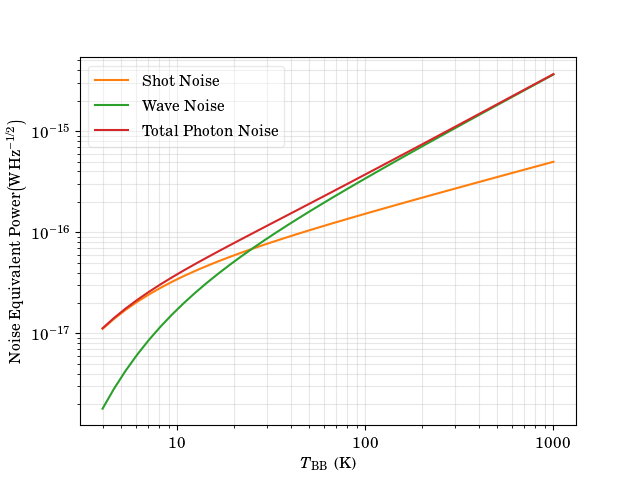
From this we see that the photon noise is dominated by the wave-noise term for any source with a temperature over approximately 25 K.

The above plot is created using the following script.

def NEPphoton(power, nu, bw, splitout=False):
    '''
    Defines the photon noise-equivalent power from both shot and wave
    noise.
    Inputs:
      power: Optical power absorbed by the detector
      nu: Central frequency of power absorbed
      bw: Optical bandwidth over which power is absorbed
      splitout:
        False: only return the total NEP (default)
        True: return the shot and wave noise values in addition to total NEP
    Output:
      (Total NEP, [shot NEP], [wave NEP]). See splitout input

    '''
    h = 6.62607E-34  # J.s
    shot = np.sqrt(2*h*nu*power)
    wave = np.sqrt(power**2/bw)
    if splitout:
        return np.sqrt(shot**2 + wave**2), shot, wave
    else:
        return np.sqrt(shot**2 + wave**2)

# Define central frequency by weighted average
nu_cent = np.average(freqFTS[idxs], weights=specFTSBBNorm[idxs])

# Create new array of temperature to explore over larger range
temps = np.logspace(np.log10(4), np.log10(1000), num=40)

P_planck = np.zeros(len(temps))
P_RJ = np.zeros(len(temps))
shot = np.zeros(len(temps))
wave = np.zeros(len(temps))
tot = np.zeros(len(temps))

for i, temp in enumerate(temps):
    P_planck = integrate.trapz(planck(freqFTS[idxs], temp)*specFTSBBNorm[idxs]*
                               AOmega, freqFTS[idxs])
    P_RJ = integrate.trapz(RJ(freqFTS[idxs], temp)*specFTSBBNorm[idxs]*AOmega,
                           freqFTS[idxs])
    tot[i], shot[i], wave[i] = NEPphoton(P_planck, nu_cent,
                                         bwHW, splitout=True)

fig, ax = plt.subplots()

ax.plot(temps, shot, label='Shot Noise')
ax.plot(temps, wave, label='Wave Noise')
ax.plot(temps, tot, label='Total Photon Noise')

Non-Planck Approximations

We can explore the effect of using the previously discussed approximations for the incident power. Below the total (quadrature some of shot and wave terms) photon noise is plotted using the Planck treatment along with the Rayleigh-Jeans and linear approximations.

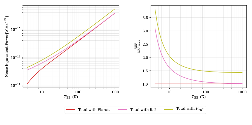
We see good agreement throughout between the Rayleigh-Jeans case and the Planck model above 100 K however the linear approximation again is an over-estimate, here by a factor of 50 % at 300 K.

These plots are produced with the following script which carries on from the previous code.

tot_RJ = np.zeros(len(temps))
tot_linear = np.zeros(len(temps))

for i, temp in enumerate(temps):
    P_planck = integrate.trapz(planck(freqFTS[idxs], temp)*specFTSBBNorm[idxs]*
                               AOmega, freqFTS[idxs])
    P_RJ = integrate.trapz(RJ(freqFTS[idxs], temp)*specFTSBBNorm[idxs]*AOmega,
                           freqFTS[idxs])
    tot_RJ[i] = NEPphoton(P_RJ, nu_cent, bwHW)
    tot_linear[i] = NEPphoton(2*kb*temp*bwHW, nu_cent, bwHW, splitout=False)

fig, [axa, axb] = plt.subplots(ncols=2, figsize=(10, 5))

axa.plot(temps, tot, label='Total with Planck')
axa.plot(temps, tot_RJ, label='Total with R-J')
axa.plot(temps, tot_linear, label='Total with KbT')

axb.plot(temps, tot/tot, label='Total with Planck')
axb.plot(temps, tot_RJ/tot, label=r'Total with R-J')
axb.plot(temps, tot_linear/tot, label=r'Total with KbT')