Spectrum and In-Band Power

The spectrum of MUSCAT's response has been measured using a Fourier Transform Spectrometer (FTS) and compares well the expected profile (Brien et al. 2018). The measured spectrum is shown below.

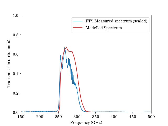
Here the modelled data consisted of the measured transmission profiles of the filters measured warm (absolute measurement) combined with the simulated performance of the horn block from HFSS.

Assumptions

The FTS measurement does not provide an absolute measure of the response spectrum. This is because it is impossible to measure the response of the detectors at a cryogenic temperature in the absence of the filters etc. (the system would not cool).

1. The 'FTS Measured' plot has been normalised to the maximum of the 'Modelled Spectrum'.
2. The 'FTS Measured' plot has also been corrected by the profile of the black body source used (1200 K).

Data Availability

The data used for the above plot are available for download here. Note the FTS data is raw data and does not have the assumptions mentioned above applied. Data are saved as ASCII encoded binary numpy arrays wrapped in dictionaries following Python 3 defaults.

• Modelled Spectrum
• FTS Measured Spectrum

FTS Analysis Script

A simple script to produce the plot shown above is:

import numpy as np
import matplotlib.pylab as plt

dataFTS = np.load('MUSCAT_band_FTS.npy')
dataModel = np.load('MUSCAT_band_model.npy')

specFTS = dataFTS.item()['spectrum']
freqFTS = dataFTS.item()['frequency']

specMod = dataModel.item()['spectrum']
freqMod = dataModel.item()['frequency']

def planck(nu, T):
    '''
    Defines Planck function in frequency space
    inputs:
      nu: Frequency in Hertz
      T: Temperature in Kelvin
    output:
      B: Spectral radiance in W m^-2 sr^-1 Hz^-1
    '''
    h = 6.62607E-34  # J.s
    kb = 1.380649E-23  # J/K
    c = 299792458  # m/s
    B = 2*h*nu**3/c**2 * 1 / (np.exp((h*nu)/(kb*T)) - 1)
    return B


# Ignore artefacts well out of band
idxs = np.where(np.logical_and(freqFTS > 150E9, freqFTS < 450E9))[0]

# Normalise for thermal source profile
specFTSBB = specFTS/planck(freqFTS, 1200)
specFTSBBNorm = specFTSBB/np.max(specFTSBB[idxs]) * np.max(specMod)
specFTSBBNorm[np.isnan(specFTSBBNorm)] = 0.  # First point will be NaN otherwise

fig1, ax1 = plt.subplots()
ax1.plot(freqMod, specMod, label='Modelled Spectrum')
ax1.plot(freqFTS, specFTSBBNorm, label='FTS Measured Spectrum')

In-Band Power

From this, the total in band power can be calculated relatively simply.

Assumptions

1. We assume that the horn block is only coupling in a single mode (as designed) and thus the throughout product, AΩ, can be expressed as the square of the designed wavelength.
2. The following example is for a black-body type source filling the detector's field of view.

Following on from the script above, the in-band power can be calculated by:

import scipy.integrate as integrate

AOmega = 1.1E-3**2  # lambda squared from design
BBBandPlanck = planck(freqFTS[idxs], 300)*specFTSBBNorm[idxs]*AOmega
powerPlanck = integrate.trapz(BBBandPlanck, freqFTS[idxs])

Which gives a value of 200 pW for the 300-K source used here.

Power Using Non-Planck Approximations

While the full Planck treatment should yield the most accurate calculation of the in-band power, it is possible to use approximations of the Planck function. The two most common of these both are based on the fact that the MUSCAT band is at much lower frequency than the peak of the black body (the Rayleigh-Jeans regime). To test these approximations we can compare the ratio of the approximated power to the power calculated using the Planck function. Here two approximations are used. Firstly, using the: Rayleigh-Jeans Law

The second case is a simple assumption that the power is linear with source temperature:

Here is the bandwidth of the spectral response. A standard treatment to calculate this would be to take the full width of the curve at half maximum the maximum value (FWHM). However, looking at the above figure we see that our response spectrum is heavily skewed to the low-frequency side and using the FWHM gives a bandwidth of 35 GHz and omits a large amount of the response. To address this, in addition to the FWHM bandwidth we also consider the bandwidth calculated using the full width at quarter the maximum value (FWQM) which gives a value of 50 GHz.

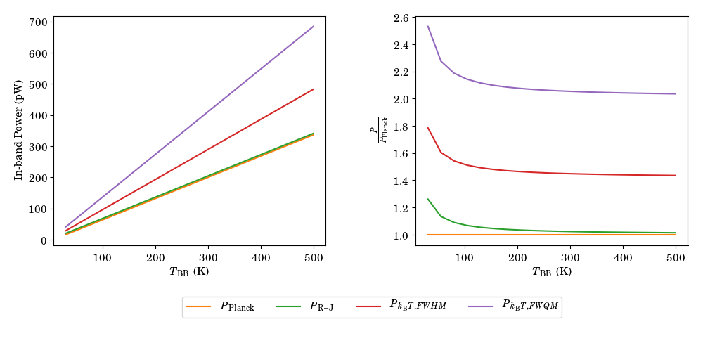
From the above figure we can see that above approximately 200 K the Rayleigh-Jeans approximation is in good agreement with the Planck function. However, the linear approximation () substantially over-estimates the power regardless of how the bandwidth is calculated.

The above plot is produce with the following script, in which variable definitions follow on the from the examples above.

def RJ(nu, T):
    '''
    Defines Rayleigh-Jeans approximation in frequency space
    inputs:
      nu: Frequency in Hertz
      T: Temperature in Kelvin
      output:
        B: Spectral radiance in W m^-2 sr^-1 Hz^-1
    '''
    kb = 1.380649E-23  # J/K
    c = 299792458  # m/s
    B = 2*nu**2*kb*T/c**2
    return B

kb = 1.380649E-23  # J/K

# Define the bandwidths
bwHM_idx = np.where(specFTSBBNorm[idxs] > np.max(specFTSBBNorm[idxs])/2)[0]
bwHM = (freqFTS[idxs][bwHM_idx[-1]] - freqFTS[idxs][bwHM_idx[1]])

bwQM_idx = np.where(specFTSBBNorm[idxs] > np.max(specFTSBBNorm[idxs])/4)[0]
bwQM = (freqFTS[idxs][bwQM_idx[-1]] - freqFTS[idxs][bwQM_idx[1]])

# List of temperatures to calculate power at
temps = np.linspace(30, 500, num=20)

P_planck = np.zeros(len(temps))
P_RJ = np.zeros(len(temps))

for i, temp in enumerate(temps):
    P_planck[i] = integrate.trapz(planck(freqFTS[idxs], temp) *
                                  specFTSBBNorm[idxs]*AOmega, freqFTS[idxs])
    P_RJ[i] = integrate.trapz(RJ(freqFTS[idxs], temp) *
                              specFTSBBNorm[idxs]*AOmega, freqFTS[idxs])

fig2, [ax2a, ax2b] = plt.subplots(ncols=2)

ax2a.plot(temps, P_planck, label='Planck')
ax2a.plot(temps, P_RJ, label='R-J')
ax2a.plot(temps, 2*kb*temps*bwHM, label='Linear, FWHM')
ax2a.plot(temps, 2*kb*temps*bwHM, label='Linear, FWQM')

ax2b.plot(temps, P_planck/P_planck)
ax2b.plot(temps, P_RJ/P_planck)
ax2b.plot(temps, 2*kb*temps*bwHM/P_planck)
ax2b.plot(temps, 2*kb*temps*bwQM/P_planck)